The US Labor Market Cools Very Slightly in June

US labor-market tightness drops from 1.7 to 1.6 in June 2023. It remains above the efficient level of 1.

The US labor-market numbers for June 2023 came out this week. This post uses the latest numbers on vacant jobs and unemployed workers from the Bureau of Labor Statistics to compute three key statistics:

• Labor-market tightness

• Efficient unemployment rate

• Unemployment gap

We also discuss monetary policy, the Beveridge curve, and the Phillips curve.

New developments

The US statistics for June 2023 are as follows:

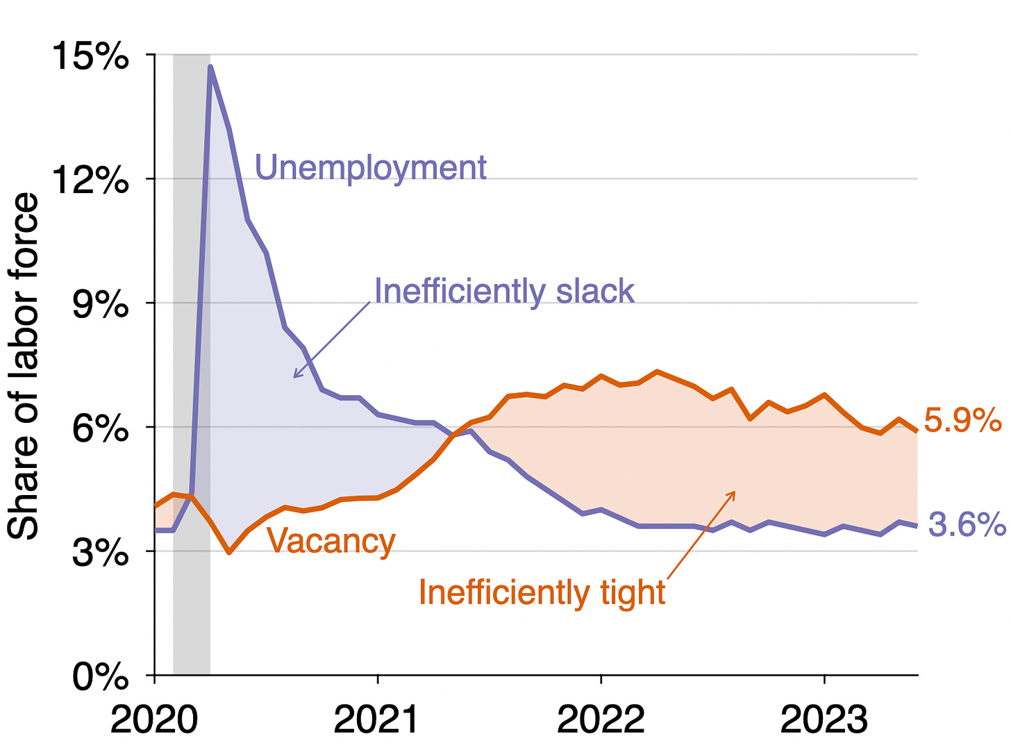
• Unemployment rate: u = 3.6%. This is down from 3.7% in May 2023.

• Vacancy rate: v = 5.9%. This is down from 6.2% in May 2023.

• Labor-market tightness: v/u = 5.9/3.6 = 1.6. This is down from 1.7 in May 2023.

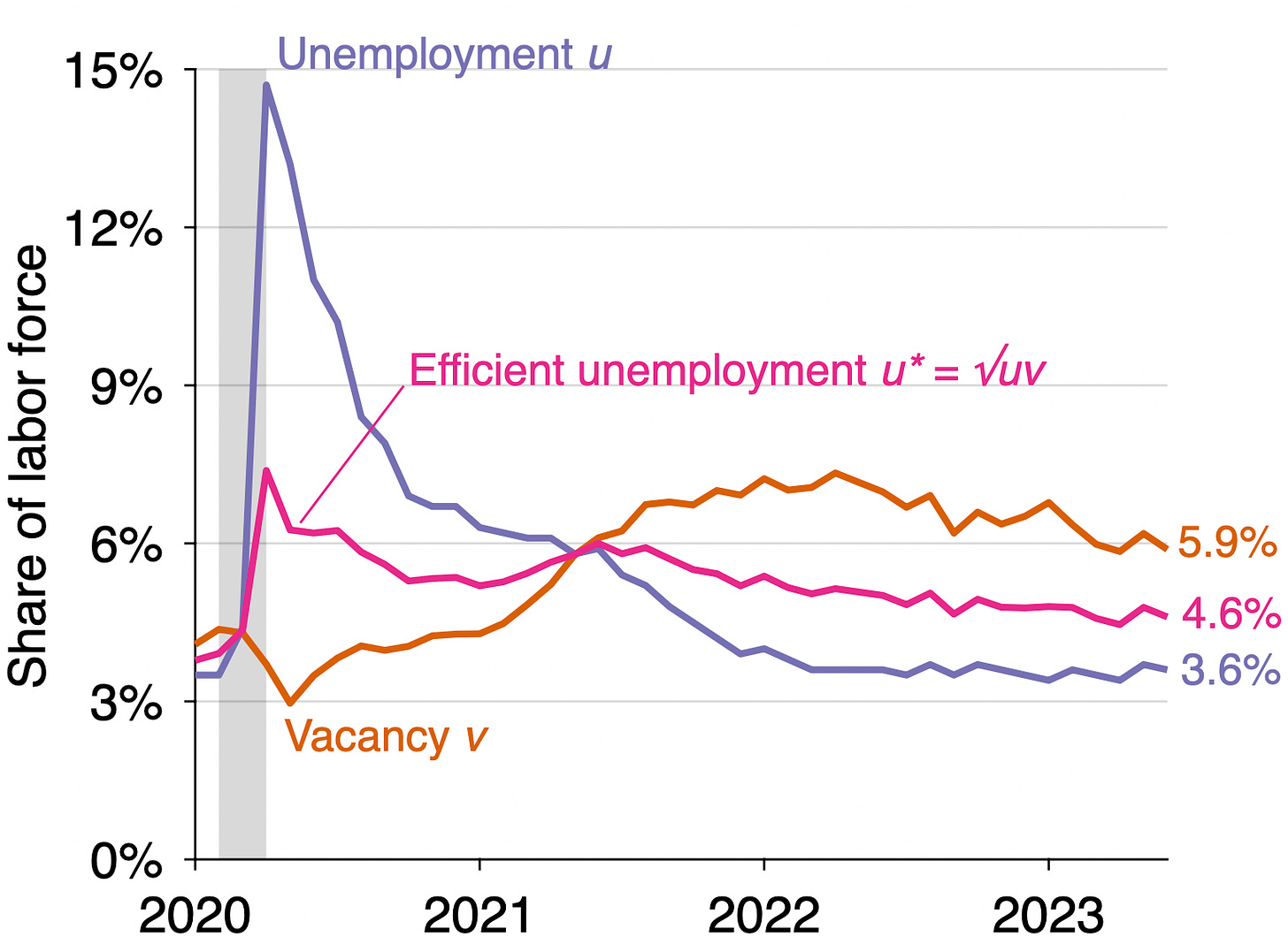
• Efficient unemployment rate: u* = √uv = √(0.036 × 0.059) = 4.6%. This is down from 4.8% in May 2023.

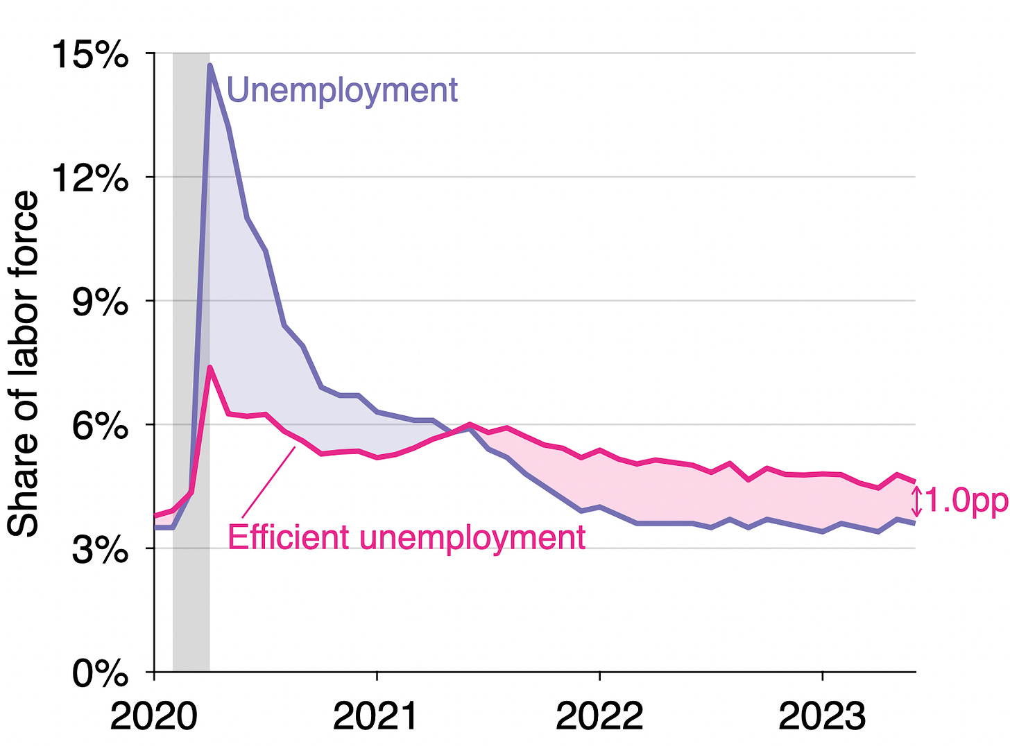
• Unemployment gap: u – u* = 0.036 – 0.046 = –1.0pp. The gap narrowed from –1.1pp in May 2023.

Is the US labor market is too tight or too slack?

Since the vacancy rate is above the unemployment rate (5.9% > 3.6%), the US labor market remains inefficiently tight. The labor market has been inefficiently tight since May 2021, as illustrated below:

We can also see that the US labor market is inefficiently tight by looking at labor-market tightness v/u, which remains above unity (1.6 > 1):

How far is unemployment from its efficient rate?

Tightness moved slightly closer to 1 in June, so the labor market moved slightly closer to efficiency. But the labor market is still inefficiently tight. This means that the actual unemployment rate remains below the efficient unemployment rate. The graph below illustrates the construction of the efficient unemployment rate:

In June 2023 the efficient unemployment rate is 1 percentage point above the actual unemployment rate (u* = 4.6% while u = 3.6%). This negative unemployment gap is another manifestation of an inefficiently tight labor market.

The efficient unemployment rate has decreased slightly from the previous month (from u* = 4.8% to u* = 4.6%) due to a slight inward shift of the Beveridge curve.

Below is the evolution of the unemployment gap over the course of the pandemic. The unemployment gap has been negative (u* > u) since the middle of 2021:

What is happening to the Beveridge curve?

The Federal Reserve has has often said that it does not expect the unemployment rate to increase much once the economy has stabilized—staying below 4%, just as it was before the pandemic when labor-market tightness was at 1.

However, as the the Fed tightens monetary policy, the labor market moves along a downward-sloping Beveridge curve. As labor-market tightness falls, the unemployment rate increases. And since the Beveridge curve shifted outward during the pandemic, it is not possible to come back to the same tightness and same unemployment rate as before the pandemic. With the pandemic curve, either tightness will be higher than before the pandemic, or unemployment will be higher.

Therefore, a soft landing can only occur if the Beveridge curve shifts back inward to its pre-pandemic location. Such shifts do not occur very often, but the curve is currently between its pre-pandemic and pandemic locations, so a shift might be in progress. Let’s keep an eye on the curve in the next few months to see whether a soft landing materializes:

What does this mean for inflation?

The concept of efficiency used in this post is based purely on the allocation of labor across producing, recruiting, and jobseeking activities. The labor market is operating efficiently when the allocation of labor across all three activities is optimal. One of the goals of the Fed is to bring the labor market to efficiency.

The other goal of the Fed is to maintain inflation around 2% per year. In a new paper, Pierpaolo Benigno and Gauti Eggertsson find that the two goals might be connected. They argue that the inefficiently high tightness experienced by the US labor market in the past 2 years might have implications for inflation through the Phillips curve.

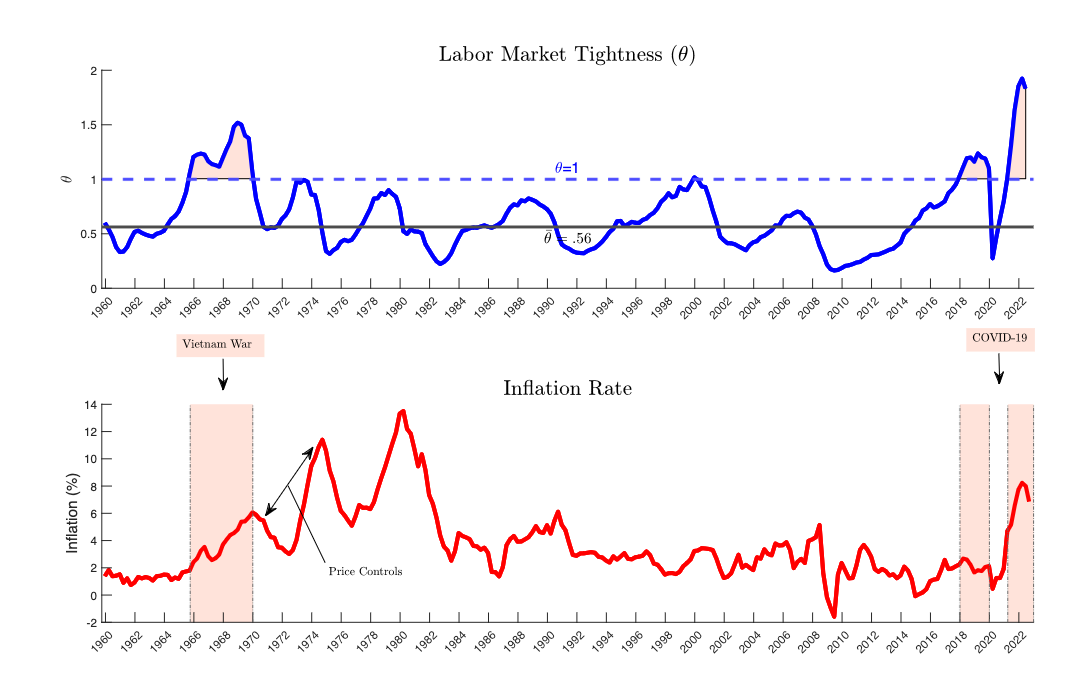
The US labor market is inefficiently tight only on very rare occasions. Since 1930, the labor market has only been too tight at the end of World War 2, during the Korean War, during the Vietnam War, and in the pandemic period. You can see this is in figure 12 from our recent paper with Emmanuel Saez:

What Pierpaolo and Gauti notice is that years when tightness is inefficiently high are also years of high inflation! This is figure 3 in their paper:

More formally, Pierpaolo and Gauti find that the Phillips curve, which relates labor-market tightness to inflation, has a kink around the efficient tightness of 1. When labor-market tightness is inefficiently low (below 1), inflation is stable. In the most recent period (2008–2022), inflation is stable around 2%, thus satisfying the Fed’s price mandate. When labor-market tightness is inefficiently high (above 1), things are very different: inflation steeply increases with tightness. The kinked Phillips curve appears in figure 4 of their paper, where the y-axis is annual CPI inflation and the x-axis is labor-market tightness v/u:

Pierpaolo and Gauti’s results imply that the divine coincidence might hold in the United States: when the labor market operates efficiently (v/u = 1), inflation reaches its target (𝛑 = 2%). This property would greatly simplify the task of the Fed. To achieve their employment and price mandates, the Fed would only need to adjust interest rates to bring labor-market tightness to 1. Then through the Phillips curve, inflation would converge to 2%.

The Fed’s dual mandate could therefore be subsumed into a single tightness mandate. To achieve both 2% inflation and full employment, the Fed would only need to maintain labor-market tightness at 1.

Background for those just joining us: data

The number of vacant jobs is measured by the Job Openings and Labor Turnover Survey (JOLTS). The number of unemployed workers is measured by the Current Population Survey (CPS). The CPS also reports the number of labor-force participants. These numbers then give unemployment and vacancy rates:

• Unemployment rate = # unemployed workers / # labor-force participants

• Vacancy rate = # vacant jobs / # labor-force participants

Background for those just joining us: methodology

The formula u* = √uv for the efficient unemployment rate is derived in a recent paper that Emmanuel Saez and I wrote. The paper shows that under simple but realistic assumptions, the efficient unemployment rate is the geometric average of the unemployment and vacancy rates—that is, u* = √uv.

An implication of this formula is that the labor market is efficient whenever there are as many unemployed workers as vacant jobs (u = v); inefficiently tight whenever there are fewer unemployed workers than vacant jobs (u < v); and inefficiently slack whenever there are more unemployed workers than vacant jobs (u > v). This criterion can also be formulated using labor-market tightness v/u.

The figures in this post are updated versions of those in the paper.