Finding the Efficient Unemployment Rate
This week's lecture material from ECON2800–Economic Slack.
There is always some slack in the economy. Sometimes there is far too much of it—for instance during the Great Recession— and sometimes there is too little of it—in the aftermath of the coronavirus pandemic for instance. I am currently teaching a PhD course on the topic at Brown University. Lecture videos, lecture notes, and readings are publicly available online.
Today’s post provides a brief overview of the material covered in this week’s lecture—which is titled “Social Welfare, Efficiency, and Inefficiency”.
Overview of this week’s lecture
The model of slack developed in the course is generally inefficient. Except in a knife-edge case, there is either too much slack or too little slack. This property arises because all the markets in the model have a matching structure. It sets the model apart from real business-cycle models, in which the economy always operates efficiently because markets are perfectly competitive, and from New Keynesian models, in which the economy is always excessively slack because markets are monopolistically competitive.
Starting from the idea that the economy might be inefficiently slack or tight, we would like to develop an empirical criterion to assess in real time whether the economy is too slack or too tight. This is what we do this week. We obtain a simple formula for the efficient unemployment rate: u* = √uv. Comparing this efficient unemployment rate to the actual unemployment rate, we find that the US labor market is generally inefficiently slack, and especially exceedingly slack in slumps.
Breakdown of this week’s lecture videos
This week’s first lecture video provides a quick introduction to the notions of social welfare and efficiency. In the analysis we will assume that welfare is simply determined by the numbers of workers devoted to production in the economy (as opposed to recruiting or jobseeking). An efficient allocation of labor between producing, recruiting, and jobseeking is an allocation that maximizes welfare.
The next lecture video discusses the concept of efficient unemployment rate. It is the unemployment rate that maximizes social welfare. This concept corresponds to what policymakers call “full employment.”
The following lecture video introduces the concept of sufficient statistics. The discussion is based on Raj Chetty’s survey of the topic. We follow the sufficient-statistic approach in this lecture, in that we make the minimal amount of structural assumptions possible to determine the efficient unemployment rate.
In the next video we introduce the only structural assumption required in the analysis: that the number of jobseekers and recruiters are negatively related through an hyperbolic Beveridge curve.
Maximizing welfare is equivalent to minimizing the number of recruiters and jobseekers. Because of the Beveridge curve, it is not desirable to bring the number of jobseekers to zero. Instead, as we show in the following lecture video, there is a positive efficient unemployment rate u*. It is the geometric average of the unemployment and vacancy rates: u* = √uv.
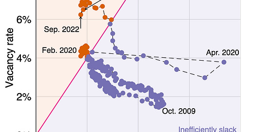
An implication of the analysis, described in the next video, is that the labor market is inefficiently slack whenever there are more jobseekers than vacancies; inefficiently tight whenever there are more vacancies than jobseekers; and efficient when there are as many jobseekers as vacancies.
In the next video, we apply this efficiency criterion to the US labor market. We find that since 1930 the unemployment rate is generally above the vacancy rate so the US labor market is generally too slack. Before the pandemic the only periods when the US labor market was too tight were wars—WW2, Korea War, Vietnam War. The US labor market has also been exceedingly tight since May 2021.
In the final video, we compute the efficient unemployment rate in the United States. The efficient unemployment rate averages 4.2% between 1930 and 2022. It has been very stable, slowly fluctuating between 3% and 5%. But it spiked above 5% in the aftermath of the pandemic due to the large outward shift of the Beveridge curve in April 2020.
This week’s readings
The analysis in this week’s lecture follows a recent paper that Emmanuel Saez and I wrote and that is titled “u* = √uv”. The paper derives the result that under simple but realistic assumptions, the efficient unemployment rate is the geometric average of the unemployment and vacancy rates: u* = √uv. The paper also applies the formula to the US labor market between 1930 and 2022.
The formula u* = √uv is based on three simplifying assumptions:
that the Beveridge curve is an hyperbola,
that unemployment is completely wasteful,
and that it takes one recruiter to service a vacancy.
These assumptions are quite realistic in the United States. Nevertheless, it is possible to obtain a much more general formula for the efficient unemployment rate—a formula that allows for any slope of the Beveridge curve, any cost of unemployment, and any recruiting cost. Emmanuel and I derive such a formula in a paper titled “Beveridgean Unemployment Gap”. In practice, the more general formula produces an efficient unemployment rate that is quite close to √uv.
Plan for next week
Next week we will discuss how monetary policy should respond to fluctuations in unemployment. We have seen this week that the unemployment rate is generally inefficient, and that it is especially inefficiently high in slumps. The extent of the inefficiency is measure by the unemployment gap—the gap between the actual unemployment rate and the efficient unemployment rate. We will see next week how the Federal Reserve can use the unemployment gap as an input to set interest rates appropriately.


