Explaining the post-pandemic inflation dynamics with a new Phillips curve

A model in which prices respond to slack instead of marginal costs explains well three key facts about post-pandemic inflation dynamics in the United States.

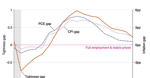
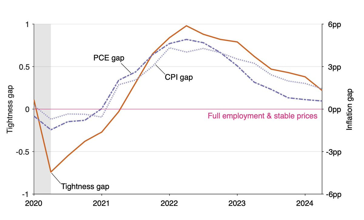
In the United States, in the aftermath of the COVID-19 pandemic, the fluctuations of inflation and labor-market slack were tightly connected, as showed in this figure:

Three key facts appear on the figure:

1. Divine coincidence: Price stability and full employment appear to coincide. Price stability is defined as an inflation rate of 2%. Full employment corresponds to a labor-market tightness (vacancy-to-unemployment ratio) of 1, as Emmanuel Saez and I show in recent work. In the graph above, the inflation gap is the deviation of inflation from 2%, and the tightness gap is the deviation of tightness from 1. The divine coincidence materializes when the tightness and inflation gaps are zero at the same time. The divine coincidence is visible in three instances: in 2020Q1, where the inflation and tightness gaps are 0; in 2021Q1–Q2, where the inflation and tightness gaps move from negative to positive and cross 0 at about the same time; and at the end of 2024, both inflation and tightness gaps are converging to 0, suggesting that the US economy will reach the point of divine coincidence again in the next few quarters.

2. Stability of the tightness-inflation Phillips curve: A version of the Phillips curve using labor-market tightness rather than unemployment is more stable. The close connection between labor-market tightness and inflation is visible on the figure as well. Tightness and inflation, whether measured from the consumer price index (CPI) or from the personal consumption expenditure (PCE) price index, evolve in tandem between 2020 and 2024. They are all at their efficient levels at the beginning of 2020: 2% for inflation and 1 for tightness. Then they all fall sharply between 2020Q1 and 2020Q2. After that they all recover, first returning to their efficient levels in 2021Q1–Q2 and then peaking well above their efficient levels in 2022Q2. Between 2022Q2 and 2024Q4, tightness and inflation have been falling, almost returning to efficiency in 2024Q2.

3. Kink at the point of divine coincidence: The Phillips curve is noticeably kinked at the point of divine coincidence, indicating that inflationary responses to labor-market changes differ depending on whether the market is tight or slack. The Phillips curve kink can be seen in the graph too. The drop in inflation between 2020Q1 and 2021Q2 is much more subdued than the coinciding drop in tightness. By contrast, the spikes in inflation and tightness between 2021Q2 and 2024Q2 have exactly the same magnitude on the scale used in the graph. This indicates that the tightness-inflation Phillips curve is much flatter when tightness is inefficiently slack than when it is inefficiently high.

These three properties—divine coincidence, stability of the tightness-inflation curve, kink—appear clearly on the graph. But Gauti Eggertsson, Pierpaolo Benigno, Giulia Gitti, Regis Barnichon, Adam Shapiro, and others have showed that the properties hold more generally and when subject to greater empirical scrutiny.

To explain these three facts, Emmanuel Saez and I develop a new, Beveridgean model of the Phillips curve. Unlike the New Keynesian model of the Phillips curve, which centers on monopolistic pricing under price-adjustment costs, our Beveridgean model operates with directed-search pricing under price-adjustment costs. We think that our model better captures real-world price adjustments. We also find that the model offers unique insights and predictions for inflation dynamics, particularly in response to labor-market shifts.

Prices driven by slack, not marginal costs

Traditional New Keynesian models link price adjustments to marginal costs, but our Beveridgean model posits that prices respond to labor-market slack instead. When the market is slack, producers face pressure to reduce prices to attract customers. Conversely, when the market is tight, producers are able to raise prices without foregoing profits. The reason—which is unique to our model—is that customers value shorter queue times and are willing to pay higher prices to have access to the goods or services more rapidly.

The shift from cost-based pricing to slack-based pricing allows the Beveridgean Phillips Curve to align better with recent inflation dynamics, as slack often captures the underlying market pressures better than marginal costs. At some level, marginal cost is an abstract concept that has no direct equivalent in the real world (this is why measuring marginal costs is so difficult and contentious). Tightness, on the other hand, is a very concrete concept, which can be measured by counting the numbers of buyers and sellers on any market, and which captures how easy or hard it is to sell or buy goods and services.

Equilibrium uniqueness and stability at the zero lower bound

One challenge in monetary models is maintaining economic stability at the zero lower bound on nominal interest rates, or when monetary policy is passive. By including wealth in the utility function, our model achieves a locally unique equilibrium that remains well-behaved even at the zero lower bound, where conventional monetary models typically fail, and even when monetary policy is passive. This approach builds on previous work with Emmanuel, in which we showed that wealth in the utility function resolves the anomalies of the New Keynesian model at the zero lower bound. Thanks to this property, the model accommodates long-lasting zero-lower-bound episodes. We can also simply assume that the Fed sets a fixed interest rate at any point in time (as they do in practice) instead of assuming that the Fed follows some Taylor rule.

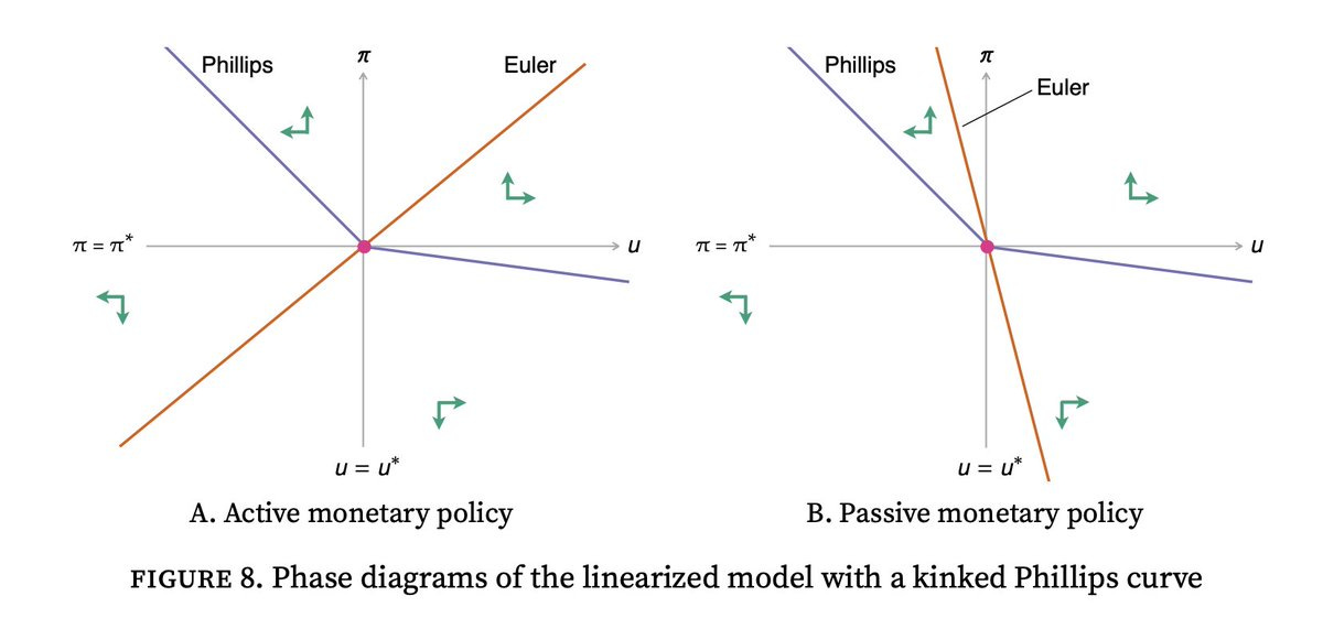
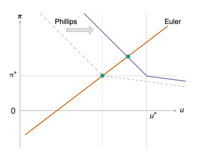
Formally, the equilibrium is always unique because the dynamical system representing the equilibrium conditions is a source whether monetary policy is active or passive, as illustrated in the phase diagrams below:

Because the system is a source, the unique equilibrium is to jump to the intersection of the Euler and Phillips curves. If the economy jumped to a different point, it would diverge to infinity, eventually violating some equilibrium constraints.

Divine coincidence

The phase diagrams above show the equilibrium in which the divine coincidence prevails. The crux is that the Phillips curve goes through the point of divine coincidence, where inflation is on target and unemployment is efficient. Then, the central bank can bring the economy to the point of divine coincidence by setting the appropriate interest rate. The interest rate chosen by the central bank moves the Euler curve along the Phillips curve. Hence, with the appropriate interest rate, the Euler curve will intersect the Phillips curve at the inflation target π* and efficient unemployment rate u*.

Accounting for shifts of the Phillips curve

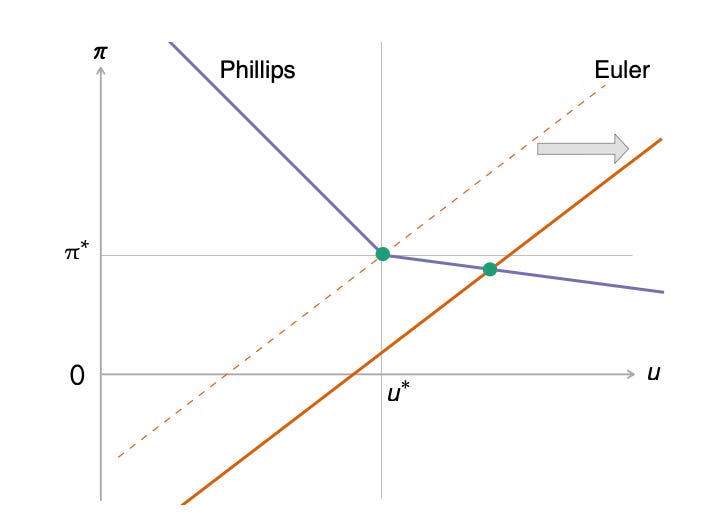
Typical business-cycle shocks are aggregate-demand shocks, which shift the Euler curve. Such shock could be caused by a change in sentiment, reflected in a different marginal utility of wealth or different discount rate. The shock could also be a change in monetary policy, affecting the nominal interest rate.

It is easy to study the effect of a negative aggregate-demand shock in the linearized model. As showed below, a negative aggregate-demand shock leads to an outward shift of the Euler curve. In response to the negative shock, unemployment is higher, the unemployment gap is also higher, and inflation is lower. The economy is moving along the Phillips curve so there is a negative correlation between unemployment and inflation. As the Phillips curve is flatter when the economy is inefficiently slack, the negative shock produces mostly an increase in unemployment. Comparatively, the drop in inflation is subdued.

Another, less common, type of shock is an aggregate-supply shock that shifts the Phillips curve. Traditional New Keynesian models often rely on “cost-push” shocks to explain sudden shifts in the Phillips curve. There is no good foundation for these cost-push shocks, which are often added in a reduced-form to the model.

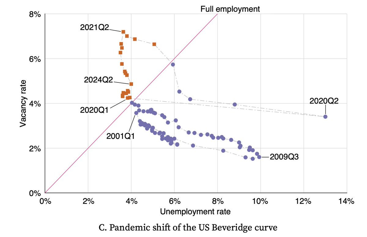
By contrast, the Beveridgean model offers a microfounded explanation for shifts in the Phillips curve by linking them to Beveridge curve movements. The Beveridge curve captures the relationship between job vacancies and unemployment. The efficient unemployment rate u* is determined by the location of the Beveridge curve. So when the Beveridge curve shifts outward, u* increases, which leads to an outward shift of the Phillips curve:

After an outward shift of the Phillips curve, inflation and unemployment rate are higher. However, whenever inflation is above target, unemployment is below its efficient level. Because the divine coincidence always holds, the inflation gap can only be positive if the unemployment gap is negative.

The situation above looks like the US economy in 2021–2024. The labor market was inefficiently tight (tightness above 1, or equivalently unemployment below u*). And inflation was above its 2% target. The cooling observed after mid 2022 is due to the Euler curve shifting outward. This outward shift reflects both the tightening of monetary policy, and the winding down of the pandemic fiscal stimulus.

The outward shift of the Phillips curve after the pandemic was caused by the dramatic outward shift of the Beveridge curve in the United States, visible here:

The Beveridge curve graph also explains why the tightness-inflation Phillips curve is more stable than the unemployment-inflation Phillips curve. The efficient tightness (represented by the pink, 45-degree line above) does not respond to shifts in the Beveridge curve. It is always 1. On the other hand, the efficient unemployment rate (represented by the intersection of the 45-degree line and Beveridge curve) does respond to shifts in the Beveridge curve. So the point of divine coincidence for the tightness-inflation Phillips curve is always (1, 2%). It is invariant to shifts in the Beveridge curve, explaining the superior stability of the tightness-inflation Phillips curve, and the superior performance of tightness in explaining inflation.

The kink and its behavioral foundations

A last feature of our Beveridgean Phillips Curve is its kink at the point of divine coincidence. In the model, the kink arises from the asymmetric impact of wage reductions and price increases. The model assumes that wage reductions, which lower worker morale, are costlier for firms than price increases, which may irritate customers. As a result, the Phillips curve steepens when the labor market is tight (because price increases are relatively less costly) and flattens when it is slack (because wage decreases are relatively more costly).

This kink has significant implications. It suggests that negative aggregate demand shocks (such as during the Great Recession) primarily increase unemployment, while negative aggregate supply shocks (as seen in the pandemic aftermath) mostly increase inflation. It also suggests that it might be easier for the Fed to target unemployment when the economy is too slack and to target inflation when the economy is too hot, because these are the most volatile variables in each regime.

Practical implications for monetary policy

The Beveridgean Phillips Curve suggests that achieving full employment naturally stabilizes inflation. It implies that policymakers can pursue full employment without risking runaway inflation. The existence of such divine coincidence is crucial for central banks like the Federal Reserve that aim to balance full employment with price stability. It implies that the dual mandate is actually achievable.

For a deeper dive into our new, Beveridgean model of the Phillips curve and its implications, see our full paper: Beveridgean Phillips Curve. For a comparison with the traditional, New Keynesian model of the Phillips curve, see our previous work: Resolving New Keynesian Anomalies with Wealth in the Utility Function.